PCNtoolkit Background
What is the PCNtoolkit?
Predictive Clinical Neuroscience (PCN) toolkit (formerly nispat) is a python package designed for multi-purpose tasks in clinical neuroimaging, including normative modelling, trend surface modelling in addition to providing implementations of a number of fundamental machine learning algorithms.
Intro to normative modelling
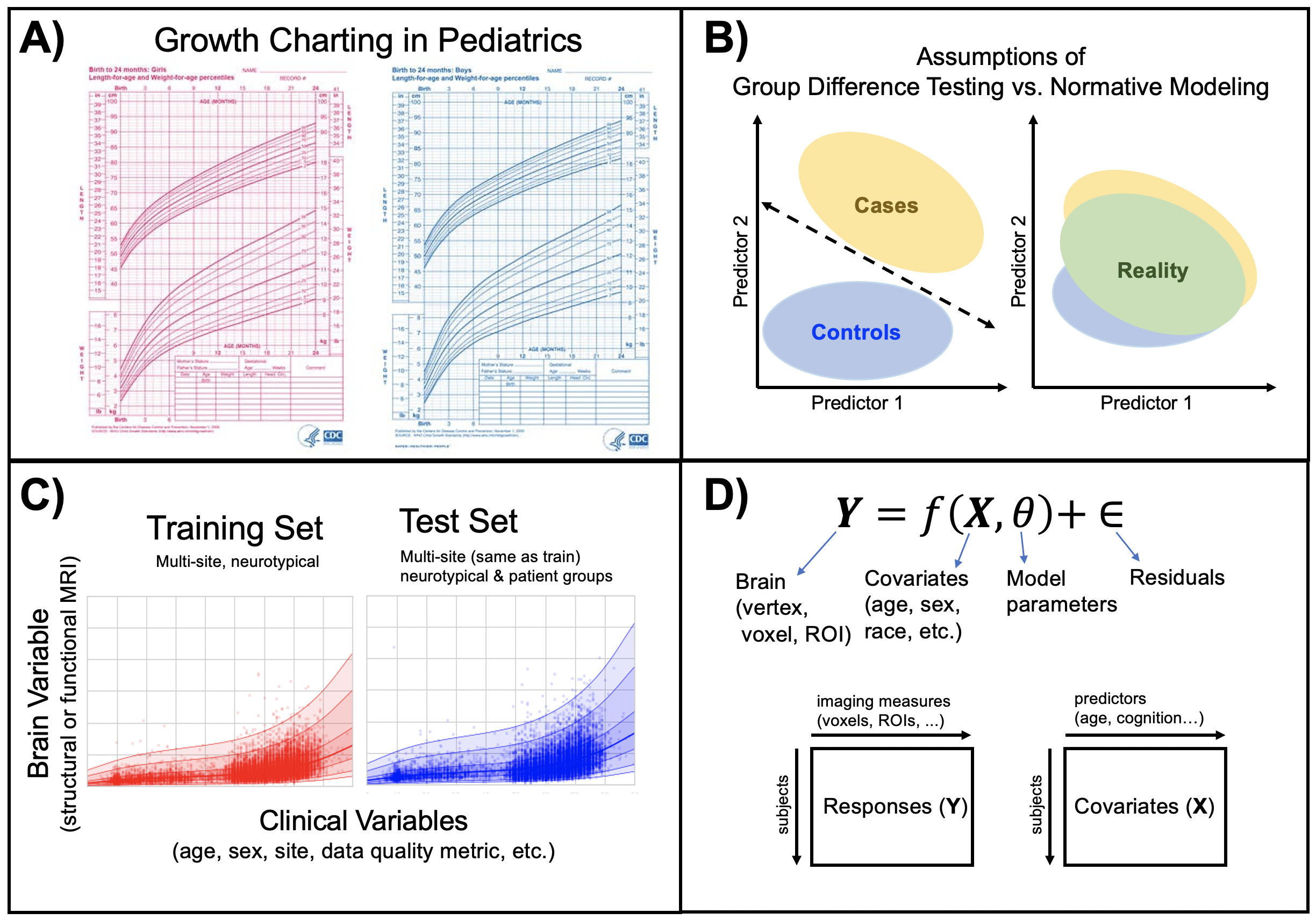
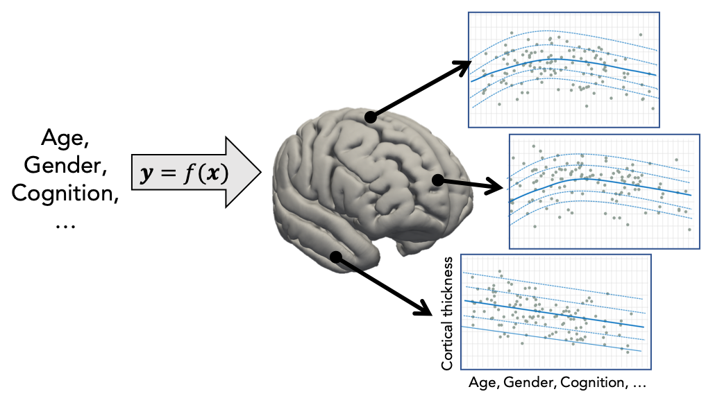
Normative modelling essentially aims to predict centiles of variance in a response variable (e.g. a region of interest or other neuroimaging-derived measure) on the basis of a set of covariates (e.g. age, clinical scores, diagnosis) A conceptual overview of the approach can be found in this publication. For example, the image below shows an example of a normative model that aims to predict vertex-wise cortical thickness data, essentially fitting a separate model for each vertex.
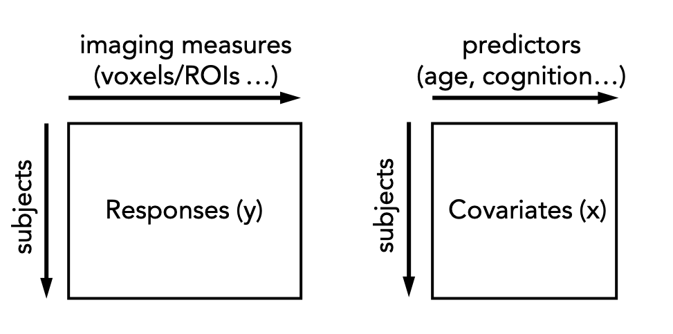
In practice, this is done by regressing the biological response variables against a set of clinical or demographic covariates. In the instructions that follow, it is helpful to think of these as being stored in matrices as shown below:
There are many options for this, but techniques that provide a distributional form for the centiles are appealing, since they help to estimate extreme centiles more efficiently. Bayesian methods are also beneficial in this regard because they also allow separation of modelling uncertainty from variation in the data. Many applications of normative modelling use Gaussian Process Regression, which is the default method in this toolkit. Typically (but not always), each response variable is estimated independently.
Data formats
Generally the covariates are specified in text format, roughly following the FSL convention in that the text file should contain one entry (i.e. subject) per line, with columns space or tab separated and no headers. For example:
head cov.txt
52 55 94 4.6
49 43 59 4.6
56 80 63 5.6
39 48 42 4.3
For the response variables, the following data formats are supported:
NIfTI (e.g. .nii.gz or .img/.hdr)
CIFTI (e.g. .dtseries.nii)
Pickle/pandas (e.g. .pkl)
ASCII text (e.g. .txt, .csv, .tsv)
For nifti/cifti formats, data should be in timeseries format with subjects along the time dimension and these images will be masked and reshaped into vectors. If no mask is specified, one will be created automatically from the image data.
Basic usage (command line)
The simplest method to estimate a normative model is using the normative.py script which can be run from the command line or imported as a python module. For example, the following command will estimate a normative model on the basis of the matrix of covariates and responses specified in cov.txt and resp.txt respectively. These are simply tab or space separated ASCII text files that contain the variables of interest, with one subject per row.
python normative.py -c cov.txt -k 5 -a blr resp.txt
The argument -a blr tells the script to use Bayesian Linear regression rather than the default Gaussian process regression model and -k 5 tells the script to run internal 5-fold cross-validation across all subjects in the covariates and responses files. Alternatively, the model can be evaluated on a separate dataset by specifying test covariates (and optionally also test responses).
The following estimation algorithms are supported
Table 1: Estimation algorithms
key value |
Description |
Reference |
hbr |
Hierarchical Bayesian Regression |
|
blr |
Bayesian Linear Regression |
|
np |
Neural Processes |
|
rfa |
Random Feature Approximation |
Note that keyword arguments can also be specified from the command line to offer additional flexibility. For example, the following command will fit a normative model to the same data, but without standardizing the data first and additionally writing out model coefficients (this is not done by default because they can use a lot of disk space).
python normative.py -c cov.txt -k 5 -a blr resp.txt standardize=False savemodel=True
A full set of keyword arguments is provided in the table below. At a minimum, a set of responses and covariates must be provided and either the corresponding number of cross-validation folds or a set of test covariates.
Table 2: Keywords and command line arguments
Keyword |
Command line shortcut |
Description |
covfunc |
-c filename |
Covariate file |
cvfolds |
-k num_folds |
Number of cross-validation folds |
testcov |
-t filename |
Test covariates |
testresp |
-r filename |
Test responses |
maskfile |
-m filename |
mask to apply to the response variables (nifti/cifti only) |
alg |
-a algorithm |
Estimation algorithm: ‘gpr’ (default), ‘blr’, ‘np’, ‘hbr’ or ‘rfa’. See table above. |
function |
-f function |
function to call (estimate, predict, transfer, extend). See below |
standardize |
-s (skip) |
Standardize the covariates and response variables using the training data |
configparam |
-x config |
Pass the value of config to the estimation algorithm (deprecated) |
outputsuffix |
Suffix to apply to the output variables |
|
saveoutput |
Write output (default = True) |
|
savemodel |
Save the model coefficients and meta-data (default = False) |
|
warp |
Warping function to apply to the responses (blr only) |
Basic usage (scripted)
The same can be done by importing the estimate function from normative.py. For example, the following code snippet will: (i) mask the nifti data specified in resp_train.nii.gz using the mask specified (which must have the same voxel size as the response variables) (ii) fit a linear normative model to each voxel, (iii) apply this to make predictions using the test covariates and (iv) compute deviation scores and error metrics by comparing against the true test response variables.
from pcntoolkit.normative import estimate

# estimate a normative model
estimate("cov_train.txt", "resp_train.nii.gz", maskfile="mask.nii.gz", \
        testresp="resp_test.nii.gz", testcov="cov_test.txt", alg="blr")
The estimate function does all these operations in a single step. In some cases it may be desirable to separate these steps. For example, if a normative model has been estimated on a large dataset, it may be desirable to save the model before applying it to a new dataset (e.g. from a a different site). For example, the following code snippet will first fit a model, then apply it to a set of dummy covariates so that the normative model can be plotted
from pcntoolkit.normative import estimate, predict

# fit a normative model, using training covariates and responses
# then apply to test dataset. Saved with file suffix '_estimate'
estimate(cov_file_tr, resp_file_tr, testresp=resp_file_te, \
        testcov=cov_file_te, alg='blr', optimizer = 'powell', \
        savemodel=True, standardize = False)

# make predictions on a set of dummy covariates (with no responses)
# Saved with file suffix '_predict'
yhat, s2 = predict(cov_file_dummy)
For further information, see the developer documentation. The same can be achieved from the command line, using te -f argument, for example, by specifying -f predict.
Paralellising estimation to speed things up
Normative model estimation is typically quite computationally expensive, especially for large datasets. This is exacerbated by high-resolution data (e.g. voxelwise data). For such cases normative model estimation can be paralellised across multiple compute nodes which can be achieved using the normative_parallel.py script. This involves splitting the response matrix into a set of batches, each of a specified size, i.e.:
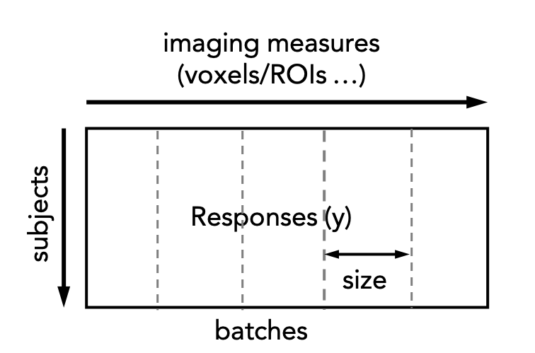
Each of these are then submitted to a cluster and reassembled once the cluster jobs have been completed. The following code snippet illustrates this procedure:
from pcntoolkit.normative_parallel import execute_nm, collect_nm, delete_nm

# General config parameters
normative_path = '/<path-to-my>/pcntoolkit/normative.py'
python_path='/<path-to-my>/bin/python'
working_dir = '/<where-results-will-be_stored>/'
log_dir = '/<where-logs-will-be_stored>/'

# cluster paramateters
job_name = 'nm_demo'   # name for the cluster job
batch_size = 10        # number of models (e.g. voxels) per batch
memory = '4gb'         # memory required
duration = '01:00:00'  # walltime
cluster = 'torque'

# fit the model. Specifying binary=True means results will be stored in .pkl format
execute_nm(working_dir, python_path, normative_path, job_name, cov_file.txt, \
        resp_file.pkl, batch_size, memory, duration, cluster_spec=cluster, \
        cv_folds=2, log_path=log_dir, binary=True)

# wait until jobs complete ...

# reassemble results
collect_nm(working_dir, job_name, collect=True, binary=True)

# remove temporary files
delete_nm(working_dir, binary=True)
At the present time, only ASCII and pickle format are supported using normative parallel. Note also that it may be necessary to customise the script to support your local cluster architecture. This can be done using fairly obvious modifications to the execute_nm() function.