Visualization of normative modeling outputs
The Normative Modeling Framework for Computational Psychiatry. Nature Protocols. https://www.nature.com/articles/s41596-022-00696-5.
Created by Saige Rutherford
We have also built an app for interactively viewing the evaluation metrics.
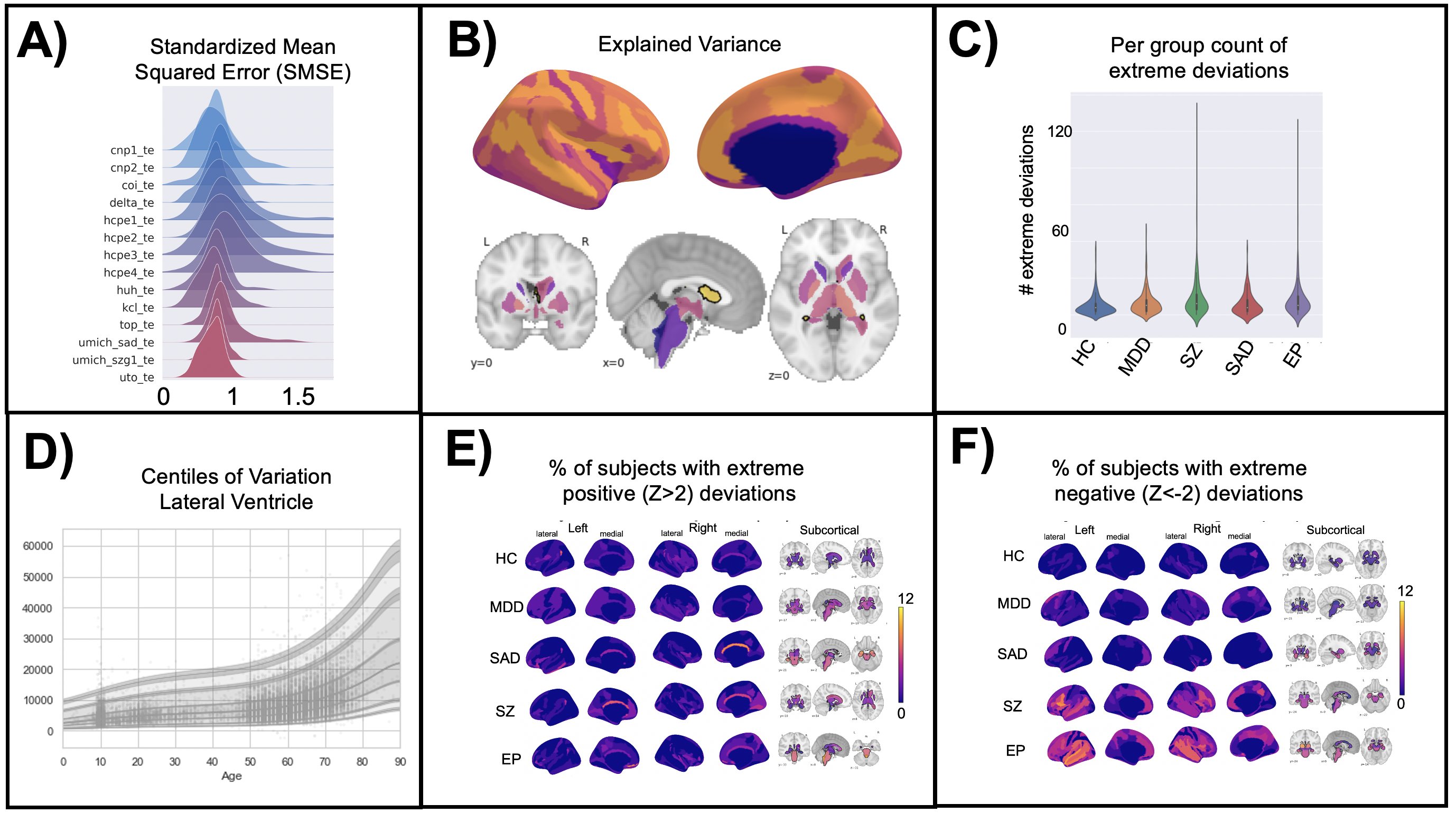
Brain space extreme deviation counts
Count the number of extreme (positive & negative) deviations at each brain region and visualize the count for each hemisphere.
! git clone https://github.com/predictive-clinical-neuroscience/PCNtoolkit-demo.git
import os
import pandas as pd
import numpy as np
import matplotlib.pyplot as plt
import seaborn as sns
os.chdir('/content/PCNtoolkit-demo')
Z_df = pd.read_csv('data/Z_long_format.csv')
# Change this threshold to view more or less extreme deviations.
# Discuss with your partner what you think is an appropriate threshold and adjust the below variables accordingly.
Z_positive = Z_df.query('value > 2')
Z_negative = Z_df.query('value < -2')
positive_left_z = Z_positive.query('hemi == "left"')
positive_right_z = Z_positive.query('hemi == "right"')
positive_sc_z = Z_positive.query('hemi == "subcortical"')
negative_left_z = Z_negative.query('hemi == "left"')
negative_right_z = Z_negative.query('hemi == "right"')
negative_sc_z = Z_negative.query('hemi == "subcortical"')
positive_left_z2 = positive_left_z['ROI_name'].value_counts().rename_axis('ROI').reset_index(name='counts')
positive_right_z2 = positive_right_z['ROI_name'].value_counts().rename_axis('ROI').reset_index(name='counts')
positive_sc_z2 = positive_sc_z['ROI_name'].value_counts().rename_axis('ROI').reset_index(name='counts')
negative_left_z2 = negative_left_z['ROI_name'].value_counts().rename_axis('ROI').reset_index(name='counts')
negative_right_z2 = negative_right_z['ROI_name'].value_counts().rename_axis('ROI').reset_index(name='counts')
negative_sc_z2 = negative_sc_z['ROI_name'].value_counts().rename_axis('ROI').reset_index(name='counts')
positive_left_z2.describe()
| counts | |
|---|---|
| count | 74.000000 |
| mean | 24.432432 |
| std | 6.182346 |
| min | 13.000000 |
| 25% | 20.000000 |
| 50% | 23.000000 |
| 75% | 28.000000 |
| max | 46.000000 |
positive_right_z2.describe()
| counts | |
|---|---|
| count | 74.000000 |
| mean | 24.027027 |
| std | 6.164354 |
| min | 11.000000 |
| 25% | 20.250000 |
| 50% | 23.000000 |
| 75% | 27.750000 |
| max | 39.000000 |
positive_sc_z2.describe()
| counts | |
|---|---|
| count | 28.000000 |
| mean | 16.714286 |
| std | 5.449140 |
| min | 8.000000 |
| 25% | 12.000000 |
| 50% | 16.000000 |
| 75% | 21.250000 |
| max | 27.000000 |
negative_left_z2.describe()
| counts | |
|---|---|
| count | 74.000000 |
| mean | 11.108108 |
| std | 5.193694 |
| min | 2.000000 |
| 25% | 7.000000 |
| 50% | 10.000000 |
| 75% | 14.000000 |
| max | 27.000000 |
negative_right_z2.describe()
| counts | |
|---|---|
| count | 74.000000 |
| mean | 12.824324 |
| std | 4.603031 |
| min | 1.000000 |
| 25% | 10.000000 |
| 50% | 13.000000 |
| 75% | 14.750000 |
| max | 33.000000 |
negative_sc_z2.describe()
| counts | |
|---|---|
| count | 28.000000 |
| mean | 9.142857 |
| std | 6.614878 |
| min | 1.000000 |
| 25% | 4.000000 |
| 50% | 7.000000 |
| 75% | 12.000000 |
| max | 26.000000 |
! pip install nilearn
from nilearn import plotting
import nibabel as nib
from nilearn import datasets
destrieux_atlas = datasets.fetch_atlas_surf_destrieux()
fsaverage = datasets.fetch_surf_fsaverage()
Dataset created in /root/nilearn_data/destrieux_surface
Downloading data from https://www.nitrc.org/frs/download.php/9343/lh.aparc.a2009s.annot ...
...done. (1 seconds, 0 min)
Downloading data from https://www.nitrc.org/frs/download.php/9342/rh.aparc.a2009s.annot ...
...done. (1 seconds, 0 min)
# The parcellation is already loaded into memory
parcellation_l = destrieux_atlas['map_left']
parcellation_r = destrieux_atlas['map_right']
nl = pd.read_csv('data/nilearn_order.csv')
atlas_r = destrieux_atlas['map_right']
atlas_l = destrieux_atlas['map_left']
nl_ROI = nl['ROI'].to_list()
Extreme positive deviation viz
nl_positive_left = pd.merge(nl, positive_left_z2, on='ROI', how='left')
nl_positive_right = pd.merge(nl, positive_right_z2, on='ROI', how='left')
nl_positive_left['counts'] = nl_positive_right['counts'].fillna(0)
nl_positive_right['counts'] = nl_positive_right['counts'].fillna(0)
nl_positive_left = nl_positive_left['counts'].to_numpy()
nl_positive_right = nl_positive_right['counts'].to_numpy()
a_list = list(range(1, 76))
parcellation_positive_l = atlas_l
for i, j in enumerate(a_list):
parcellation_positive_l = np.where(parcellation_positive_l == j, nl_positive_left[i], parcellation_positive_l)
a_list = list(range(1, 76))
parcellation_positive_r = atlas_r
for i, j in enumerate(a_list):
parcellation_positive_r = np.where(parcellation_positive_r == j, nl_positive_right[i], parcellation_positive_r)
# you can click around in 3D space on this visualization. Scroll in/out, move the brain around, etc. Have fun with it :)
view = plotting.view_surf(fsaverage.infl_right, parcellation_positive_r, threshold=None, symmetric_cmap=False, cmap='plasma', bg_map=fsaverage.sulc_right)
view
view = plotting.view_surf(fsaverage.infl_left, parcellation_positive_l, threshold=None, symmetric_cmap=False, cmap='plasma', bg_map=fsaverage.sulc_left)
view
Extreme negative deviation viz
nl_negative_left = pd.merge(nl, negative_left_z2, on='ROI', how='left')
nl_negative_right = pd.merge(nl, negative_right_z2, on='ROI', how='left')
nl_negative_left['counts'] = nl_negative_left['counts'].fillna(0)
nl_negative_right['counts'] = nl_negative_right['counts'].fillna(0)
nl_negative_left = nl_negative_left['counts'].to_numpy()
nl_negative_right = nl_negative_right['counts'].to_numpy()
a_list = list(range(1, 76))
parcellation_negative_l = atlas_l
for i, j in enumerate(a_list):
parcellation_negative_l = np.where(parcellation_negative_l == j, nl_negative_left[i], parcellation_negative_l)
a_list = list(range(1, 76))
parcellation_negative_r = atlas_r
for i, j in enumerate(a_list):
parcellation_negative_r = np.where(parcellation_negative_r == j, nl_negative_right[i], parcellation_negative_r)
view = plotting.view_surf(fsaverage.infl_right, parcellation_negative_r, threshold=None, symmetric_cmap=False, cmap='plasma', bg_map=fsaverage.sulc_right)
view
view = plotting.view_surf(fsaverage.infl_left, parcellation_negative_l, threshold=None, symmetric_cmap=False, cmap='plasma', bg_map=fsaverage.sulc_left)
view
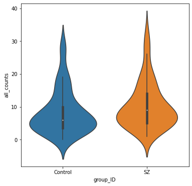
Violin plots of extreme deviations
We will count the number of “extreme” deviations that each person has (both positive and negative) and summarize the distribution of extreme deviations for healthy controls and patients with schizophrenia.
Z_df = pd.read_csv('data/fcon1000_te_Z.csv')
deviation_counts = Z_df.loc[:, Z_df.columns.str.contains('Z_predict')]
deviation_counts['positive_count'] = deviation_counts[deviation_counts >= 2].count(axis=1)
deviation_counts['negative_count'] = deviation_counts[deviation_counts <= -2].count(axis=1)
deviation_counts['participant_id'] = Z_df['sub_id']
deviation_counts['group_ID'] = Z_df['group']
deviation_counts['site_ID'] = Z_df['site']
deviation_counts['all_counts'] = deviation_counts['positive_count'] + deviation_counts['negative_count']
fig, ax = plt.subplots(figsize=(6,6))
sns.violinplot(data=deviation_counts, y="all_counts", x="group_ID", inner='box', ax=ax);
plt.legend=False
Centile visualization
The code used to visualize the centiles of variation can be found in this notebook.