Getting started with normative modelling

Welcome to this tutorial notebook that will show you the very basics of normative modeling. It’s like the “Hello World” of normative modeling.

Let’s jump right in.

Imports

import warnings
import pandas as pd
import matplotlib.pyplot as plt
from pcntoolkit import (
    BLR,
    NormativeModel,
    NormData,
    load_fcon1000,
    plot_centiles,
    plot_qq,
)
import pcntoolkit.util.output
import seaborn as sns

sns.set_style("darkgrid")
warnings.simplefilter(action="ignore", category=FutureWarning)
pd.options.mode.chained_assignment = None  # default='warn'
pcntoolkit.util.output.Output.set_show_messages(False)

Load data

First we download a small example dataset from github.

# Download an example dataset
norm_data: NormData = load_fcon1000()
# Select only these three features to model for this example
norm_data = norm_data.sel({"response_vars": ["WM-hypointensities", "Left-Lateral-Ventricle", "Brain-Stem"]})
# Train-test split
train, test = norm_data.train_test_split()

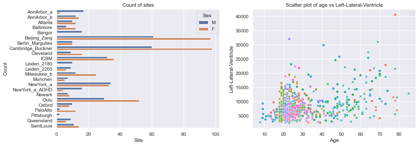
# Inspect the data
df = train.to_dataframe()
fig, ax = plt.subplots(1, 2, figsize=(15, 5))

sns.countplot(data=df, y=("batch_effects", "site"), hue=("batch_effects", "sex"), ax=ax[0], orient="h")
ax[0].legend(title="Sex")
ax[0].set_title("Count of sites")
ax[0].set_xlabel("Site")
ax[0].set_ylabel("Count")

scatter_feature = "Left-Lateral-Ventricle"

sns.scatterplot(
    data=df,
    x=("X", "age"),
    y=("Y", scatter_feature),
    hue=("batch_effects", "site"),
    style=("batch_effects", "sex"),
    ax=ax[1],
)
ax[1].legend([], [])
ax[1].set_title(f"Scatter plot of age vs {scatter_feature}")
ax[1].set_xlabel("Age")
ax[1].set_ylabel(scatter_feature)

plt.show()

Creating a Normative model

save_dir = "/Users/stijndeboer/Projects/PCN/PCNtoolkit/examples/saves"
model = NormativeModel(BLR(), inscaler="standardize", outscaler="standardize")

model.has_batch_effect

False

Fit the model

With all that configured, we can fit the model.

The fit_predict function will fit the model, evaluate it, save the results and plots, and return the test data with all the predictions added.

After that, it will compute Z-scores and centiles for the test set.

All results can be found in the save directory.

model.fit_predict(train, test)

<xarray.NormData> Size: 87kB
Dimensions:            (observations: 216, response_vars: 3, covariates: 1,
                        batch_effect_dims: 2, centile: 5, statistic: 11)
Coordinates:
  * observations       (observations) int64 2kB 756 769 692 616 ... 751 470 1043
  * response_vars      (response_vars) <U22 264B 'WM-hypointensities' ... 'Br...
  * covariates         (covariates) <U3 12B 'age'
  * batch_effect_dims  (batch_effect_dims) <U4 32B 'sex' 'site'
  * centile            (centile) float64 40B 0.05 0.25 0.5 0.75 0.95
  * statistic          (statistic) <U8 352B 'EXPV' 'MACE' ... 'SMSE' 'ShapiroW'
Data variables:
    subject_ids        (observations) object 2kB 'Munchen_sub96752' ... 'Quee...
    Y                  (observations, response_vars) float64 5kB 2.721e+03 .....
    X                  (observations, covariates) float64 2kB 63.0 ... 23.0
    batch_effects      (observations, batch_effect_dims) <U17 29kB 'F' ... 'Q...
    Z                  (observations, response_vars) float64 5kB 0.8681 ... -...
    centiles           (centile, observations, response_vars) float64 26kB 75...
    logp               (observations, response_vars) float64 5kB -1.254 ... -...
    Yhat               (observations, response_vars) float64 5kB 2.041e+03 .....
    statistics         (response_vars, statistic) float64 264B 0.1501 ... 0.9891
    Y_harmonized       (observations, response_vars) float64 5kB 2.721e+03 .....
Attributes:
    real_ids:                       True
    is_scaled:                      False
    name:                           fcon1000_test
    unique_batch_effects:           {np.str_('sex'): [np.str_('F'), np.str_('...
    batch_effect_counts:            defaultdict(<function NormData.register_b...
    covariate_ranges:               {np.str_('age'): {'mean': np.float64(28.2...
    batch_effect_covariate_ranges:  {np.str_('sex'): {np.str_('F'): {np.str_(...

xarray.NormData

• Dimensions:
  • observations: 216
  • response_vars: 3
  • covariates: 1
  • batch_effect_dims: 2
  • centile: 5
  • statistic: 11
• Coordinates: (6)
  • observations
    (observations)
    int64
    756 769 692 616 ... 751 470 1043

    array([ 756,  769,  692, ...,  751,  470, 1043], shape=(216,))

  • response_vars
    (response_vars)
    <U22
    'WM-hypointensities' ... 'Brain-...

    array(['WM-hypointensities', 'Left-Lateral-Ventricle', 'Brain-Stem'],
          dtype='<U22')

  • covariates
    (covariates)
    <U3
    'age'

    array(['age'], dtype='<U3')

  • batch_effect_dims
    (batch_effect_dims)
    <U4
    'sex' 'site'

    array(['sex', 'site'], dtype='<U4')

  • centile
    (centile)
    float64
    0.05 0.25 0.5 0.75 0.95

    array([0.05, 0.25, 0.5 , 0.75, 0.95])

  • statistic
    (statistic)
    <U8
    'EXPV' 'MACE' ... 'SMSE' 'ShapiroW'

    array(['EXPV', 'MACE', 'MAPE', 'MSLL', 'NLL', 'R2', 'RMSE', 'Rho', 'Rho_p',
           'SMSE', 'ShapiroW'], dtype='<U8')

• Data variables: (10)
  • subject_ids
    (observations)
    object
    'Munchen_sub96752' ... 'Queensla...

    array(['Munchen_sub96752', 'NewYork_a_sub18638', 'Leiden_2200_sub87320',
           'ICBM_sub47658', 'AnnArbor_b_sub45569', 'Beijing_Zang_sub18960',
           'Leiden_2200_sub18456', 'Berlin_Margulies_sub27711',
           'Beijing_Zang_sub87776', 'Milwaukee_b_sub63196',
           'Beijing_Zang_sub07144', 'Atlanta_sub76280',
           'Beijing_Zang_sub40037', 'Cambridge_Buckner_sub17737',
           'ICBM_sub89049', 'ICBM_sub55656', 'Oulu_sub45566',
           'Beijing_Zang_sub89088', 'Atlanta_sub16563',
           'Cambridge_Buckner_sub51172', 'Oulu_sub98739',
           'Queensland_sub49845', 'Cambridge_Buckner_sub84256',
           'Cleveland_sub80263', 'ICBM_sub16607', 'Newark_sub46570',
           'NewYork_a_sub88286', 'Cambridge_Buckner_sub02591',
           'Oulu_sub66467', 'Beijing_Zang_sub74386', 'Newark_sub55760',
           'ICBM_sub30623', 'Oulu_sub68752', 'Leiden_2180_sub19281',
           'Beijing_Zang_sub50972', 'Beijing_Zang_sub85030',
           'Milwaukee_b_sub36386', 'Baltimore_sub31837', 'PaloAlto_sub84978',
           'Oulu_sub01077', 'NewYork_a_ADHD_sub54828', 'PaloAlto_sub96705',
           'Cambridge_Buckner_sub40635', 'ICBM_sub66794',
           'Beijing_Zang_sub46541', 'Beijing_Zang_sub87089',
           'Pittsburgh_sub97823', 'Beijing_Zang_sub98617', 'ICBM_sub92028',
    ...
           'Leiden_2200_sub04484', 'Beijing_Zang_sub80163', 'ICBM_sub02382',
           'Cambridge_Buckner_sub77435', 'NewYork_a_sub54887',
           'Oulu_sub85532', 'Baltimore_sub73823', 'Beijing_Zang_sub29590',
           'Oulu_sub99718', 'Beijing_Zang_sub08455', 'Beijing_Zang_sub85543',
           'Cambridge_Buckner_sub45354', 'Beijing_Zang_sub07717',
           'Baltimore_sub76160', 'Beijing_Zang_sub17093',
           'AnnArbor_b_sub90127', 'SaintLouis_sub73002',
           'Queensland_sub93238', 'Cleveland_sub34189',
           'Cambridge_Buckner_sub89107', 'Atlanta_sub75153',
           'NewYork_a_ADHD_sub73035', 'Cambridge_Buckner_sub59434',
           'Milwaukee_b_sub44912', 'Cleveland_sub46739', 'Oulu_sub20495',
           'SaintLouis_sub28304', 'Cambridge_Buckner_sub35430',
           'Oulu_sub86362', 'Newark_sub58526', 'Leiden_2180_sub12255',
           'ICBM_sub48210', 'Cambridge_Buckner_sub77989',
           'Berlin_Margulies_sub75506', 'NewYork_a_sub29216',
           'Beijing_Zang_sub05267', 'AnnArbor_b_sub18546', 'Oulu_sub75620',
           'AnnArbor_b_sub30250', 'Berlin_Margulies_sub86111',
           'Beijing_Zang_sub89592', 'Beijing_Zang_sub68012',
           'NewYork_a_sub50559', 'Munchen_sub66933',
           'Cambridge_Buckner_sub59729', 'Queensland_sub86245'], dtype=object)

  • Y
    (observations, response_vars)
    float64
    2.721e+03 1.362e+04 ... 1.681e+04

    array([[ 2721.4, 13617.8, 22653.2],
           [ 1143.1, 10922.3, 20821.3],
           [  955.8,  8374.3, 19278.9],
           [ 1473.9, 16068.7, 25724. ],
           [  757.8,  4107.1, 16570.4],
           [  871.1,  5962.5, 23831.3],
           [ 1207.3, 19877.6, 23995.9],
           [  595. ,  5568.6, 21180.8],
           [  682.4,  6953.8, 15396.4],
           [  445.1,  6771.1, 20429.1],
           [ 1620. ,  3980.3, 21843.1],
           [  602.8,  6051.4, 19098.4],
           [ 1432.5,  5916.8, 22060.2],
           [ 1908.2,  4656.4, 22974.4],
           [ 1834. ,  3691.9, 26658.4],
           [  459.6,  5823.6, 21087. ],
           [ 1210. ,  6667.1, 23873.9],
           [  845.9,  7648.6, 20948.3],
           [  995.2,  6850.1, 20345.2],
           [ 1734.7,  4457. , 18642.8],
    ...
           [  785.8,  6197.9, 20216. ],
           [ 2240.1,  4806.6, 27596.4],
           [  758.1,  5615.1, 24054.6],
           [ 1440.5,  7500.1, 13773.6],
           [  818.6,  9928.8, 21445.7],
           [ 3769.9, 19406.4, 23748.4],
           [  880.2,  7366.4, 21144.5],
           [  823.9, 11342.3, 25405.8],
           [ 2113.9,  8920.5, 22618.7],
           [  741.9, 11228.2, 20471.4],
           [ 1333.9,  9730.4, 22427.1],
           [  707.3,  6458.2, 21449.5],
           [ 1134.1,  6038.2, 15343. ],
           [  438.6,  7505.7, 15679.7],
           [  966.3, 10570. , 19890.2],
           [  424.3,  4887. , 21624.5],
           [  604.7,  8933.9, 18852.1],
           [ 2343.2, 19039.7, 18791.2],
           [ 2721.7,  4899.1, 23784.8],
           [  703.5, 10060.7, 16805.6]])

  • X
    (observations, covariates)
    float64
    63.0 23.27 22.0 ... 72.0 23.0 23.0

    array([[63.  ],
           [23.27],
           [22.  ],
           [42.  ],
           [63.  ],
           [23.  ],
           [21.  ],
           [26.  ],
           [21.  ],
           [49.  ],
           [20.  ],
           [23.  ],
           [20.  ],
           [26.  ],
           [35.  ],
           [21.  ],
           [22.  ],
           [19.  ],
           [34.  ],
           [18.  ],
    ...
           [21.  ],
           [20.  ],
           [22.  ],
           [25.  ],
           [25.  ],
           [73.  ],
           [22.  ],
           [28.  ],
           [29.06],
           [19.  ],
           [20.  ],
           [22.  ],
           [19.  ],
           [24.  ],
           [21.  ],
           [24.  ],
           [22.79],
           [72.  ],
           [23.  ],
           [23.  ]])

  • batch_effects
    (observations, batch_effect_dims)
    <U17
    'F' 'Munchen' ... 'M' 'Queensland'

    array([['F', 'Munchen'],
           ['M', 'NewYork_a'],
           ['F', 'Leiden_2200'],
           ['M', 'ICBM'],
           ['F', 'AnnArbor_b'],
           ['M', 'Beijing_Zang'],
           ['M', 'Leiden_2200'],
           ['F', 'Berlin_Margulies'],
           ['F', 'Beijing_Zang'],
           ['F', 'Milwaukee_b'],
           ['M', 'Beijing_Zang'],
           ['F', 'Atlanta'],
           ['F', 'Beijing_Zang'],
           ['F', 'Cambridge_Buckner'],
           ['M', 'ICBM'],
           ['F', 'ICBM'],
           ['M', 'Oulu'],
           ['F', 'Beijing_Zang'],
           ['M', 'Atlanta'],
           ['F', 'Cambridge_Buckner'],
    ...
           ['F', 'SaintLouis'],
           ['M', 'Cambridge_Buckner'],
           ['F', 'Oulu'],
           ['F', 'Newark'],
           ['M', 'Leiden_2180'],
           ['M', 'ICBM'],
           ['F', 'Cambridge_Buckner'],
           ['M', 'Berlin_Margulies'],
           ['M', 'NewYork_a'],
           ['F', 'Beijing_Zang'],
           ['M', 'AnnArbor_b'],
           ['F', 'Oulu'],
           ['F', 'AnnArbor_b'],
           ['F', 'Berlin_Margulies'],
           ['M', 'Beijing_Zang'],
           ['F', 'Beijing_Zang'],
           ['M', 'NewYork_a'],
           ['M', 'Munchen'],
           ['M', 'Cambridge_Buckner'],
           ['M', 'Queensland']], dtype='<U17')

  • Z
    (observations, response_vars)
    float64
    0.8681 0.3703 ... 0.7406 -1.556

    array([[ 8.68050427e-01,  3.70323407e-01,  8.36221702e-01],
           [-3.51254255e-02,  9.48730585e-01,  8.49790658e-02],
           [-2.39376648e-01,  3.48187823e-01, -5.45562934e-01],
           [-1.37096721e-01,  1.65029723e+00,  2.09032291e+00],
           [-1.63782699e+00, -2.01209266e+00, -1.64067079e+00],
           [-3.75946561e-01, -2.89767858e-01,  1.31513122e+00],
           [ 1.10818471e-01,  3.27173916e+00,  1.38201038e+00],
           [-8.13867842e-01, -4.83584174e-01,  2.32310274e-01],
           [-5.61464250e-01,  2.26314627e-02, -2.13233893e+00],
           [-1.64935106e+00, -9.06449218e-01, -7.15750526e-02],
           [ 6.67432756e-01, -6.93307940e-01,  5.02061271e-01],
           [-7.19607720e-01, -2.67416184e-01, -6.19211599e-01],
           [ 4.27297820e-01, -2.06486071e-01,  5.90778967e-01],
           [ 8.68309390e-01, -7.12950392e-01,  9.65409569e-01],
           [ 5.20544881e-01, -1.23956846e+00,  2.47214033e+00],
           [-8.46822585e-01, -2.61506448e-01,  1.93233044e-01],
           [ 8.62121759e-02, -8.10291138e-02,  1.33235151e+00],
           [-2.95889244e-01,  2.60439063e-01,  1.36252812e-01],
           [-5.25754725e-01, -4.13996977e-01, -1.08081102e-01],
           [ 8.70362937e-01, -5.10253867e-01, -8.05927475e-01],
    ...
           [-4.29031342e-01, -1.67405563e-01, -1.62717680e-01],
           [ 1.46160702e+00, -4.85582192e-01,  2.85314152e+00],
           [-4.92598169e-01, -3.45518463e-01,  1.40620116e+00],
           [ 2.97264178e-01,  3.36612747e-02, -2.79533212e+00],
           [-4.99360583e-01,  6.44329927e-01,  3.40435211e-01],
           [ 1.92167686e+00,  1.50198108e+00,  1.28042289e+00],
           [-3.36207943e-01,  9.47859070e-02,  2.16882593e-01],
           [-5.76806544e-01,  9.05018310e-01,  1.95951278e+00],
           [ 1.04592009e+00,  2.62583905e-01,  8.20470104e-01],
           [-4.29076719e-01,  1.16027440e+00, -5.86211131e-02],
           [ 3.01018861e-01,  7.52224942e-01,  7.40712283e-01],
           [-5.57664700e-01, -1.33549860e-01,  3.41531974e-01],
           [ 7.31937396e-02, -1.44381259e-01, -2.15422068e+00],
           [-9.58028076e-01,  6.66512514e-02, -2.01635803e+00],
           [-1.97850105e-01,  9.31762157e-01, -2.95862050e-01],
           [-9.76345269e-01, -5.91774995e-01,  4.13363274e-01],
           [-7.11274199e-01,  4.63944956e-01, -7.19899399e-01],
           [ 1.33408839e-01,  1.44213468e+00, -7.33482498e-01],
           [ 1.99445724e+00, -5.57133095e-01,  1.29612660e+00],
           [-5.90622708e-01,  7.40621663e-01, -1.55628215e+00]])

  • centiles
    (centile, observations, response_vars)
    float64
    752.3 5.573e+03 ... 2.464e+04

    array([[[  752.29394222,  5573.13286211, 16560.12771737],
            [ -113.62127992,   606.84799863, 16588.82717329],
            [ -141.51115319,   447.02576072, 16589.08591226],
            ...,
            [  946.6875119 ,  6689.16629877, 16548.1078189 ],
            [ -119.54953172,   572.87560298, 16588.88560005],
            [ -119.54953172,   572.87560298, 16588.88560005]],
    
           [[ 1512.66892952,  9446.86418123, 18943.16589981],
            [  643.94570069,  4466.2723232 , 18963.06761723],
            [  616.09008872,  4306.62464909, 18963.43369989],
            ...,
            [ 1708.73771431, 10571.43295571, 18936.39460621],
            [  638.02408897,  4432.33375922, 18963.14684793],
            [  638.02408897,  4432.33375922, 18963.14684793]],
    
           [[ 2041.19760574, 12139.45418004, 20599.59073887],
            [ 1170.52256093,  7148.9176802 , 20613.37724056],
            [ 1142.69076363,  6989.39134356, 20613.81793668],
            ...,
            [ 2238.43081498, 13269.9557783 , 20596.46769545],
            [ 1164.60556465,  7115.00263226, 20613.47093186],
            [ 1164.60556465,  7115.00263226, 20613.47093186]],
    
           [[ 2569.72628196, 14832.04417885, 22256.01557793],
            [ 1697.09942117,  9831.5630372 , 22263.68686388],
            [ 1669.29143854,  9672.15803803, 22264.20217348],
            ...,
            [ 2768.12391565, 15968.47860088, 22256.54078469],
            [ 1691.18704034,  9797.67150529, 22263.79501579],
            [ 1691.18704034,  9797.67150529, 22263.79501579]],
    
           [[ 3330.10126925, 18705.77549797, 24639.05376037],
            [ 2454.66640178, 13690.98736177, 24637.92730782],
            [ 2426.89268045, 13531.7569264 , 24638.54996111],
            ...,
            [ 3530.17411806, 19850.74525782, 24644.827572  ],
            [ 2448.76066103, 13657.12966153, 24638.05626368],
            [ 2448.76066103, 13657.12966153, 24638.05626368]]],
          shape=(5, 216, 3))

  • logp
    (observations, response_vars)
    float64
    -1.254 -0.9282 ... -1.13 -2.132

    array([[ -1.25430906,  -0.92819793,  -1.27414414],
           [ -0.87447043,  -1.30597291,  -0.92442284],
           [ -0.90254934,  -0.91659065,  -1.06967679],
           [ -0.88376337,  -2.21818065,  -3.10604898],
           [ -2.21879191,  -2.88388665,  -2.27041109],
           [ -0.9445302 ,  -0.89791952,  -1.78560594],
           [ -0.88008187,  -6.20815461,  -1.87587642],
           [ -1.20498112,  -0.97279202,  -0.94773333],
           [ -1.03156256,  -0.85627212,  -3.19433473],
           [ -2.23530223,  -1.26802253,  -0.92464248],
           [ -1.09672379,  -1.09640303,  -1.04698186],
           [ -1.13277993,  -0.89169252,  -1.11253238],
           [ -0.96528226,  -0.87738333,  -1.09545899],
           [ -1.25077128,  -1.11001433,  -1.38675711],
           [ -1.00939937,  -1.62425539,  -3.97661337],
           [ -1.23249575,  -0.89020884,  -0.93956958],
           [ -0.87761502,  -0.85925613,  -1.80843761],
           [ -0.9178211 ,  -0.89003467,  -0.93028683],
           [ -1.01208581,  -0.94164806,  -0.92667614],
           [ -1.25287332,  -0.98636155,  -1.24582556],
    ...
           [ -0.96597545,  -0.87002834,  -0.93413859],
           [ -1.94213809,  -0.97396011,  -4.99115737],
           [ -0.99522523,  -0.91566478,  -1.90955819],
           [ -0.91799126,  -0.85644931,  -4.82770771],
           [ -0.99848876,  -1.0634633 ,  -0.97871493],
           [ -2.72645001,  -1.99007782,  -1.74672717],
           [ -0.93041664,  -0.86046546,  -0.94437636],
           [ -1.04012732,  -1.26537801,  -2.84057821],
           [ -1.42075045,  -0.89032569,  -1.25732024],
           [ -0.9660993 ,  -1.52923876,  -0.92272263],
           [ -0.91929673,  -1.13898626,  -1.19527644],
           [ -1.02939371,  -0.86489106,  -0.97917938],
           [ -0.87672454,  -0.86654339,  -3.2413378 ],
           [ -1.33274103,  -0.85812784,  -2.95364058],
           [ -0.89351384,  -1.29010639,  -0.96466725],
           [ -1.35045717,  -1.03100546,  -1.00622532],
           [ -1.12682492,  -0.96356641,  -1.17995559],
           [ -0.88865297,  -1.9017054 ,  -1.19570912],
           [ -2.86279214,  -1.01113545,  -1.76079297],
           [ -1.04827989,  -1.13019704,  -2.13182795]])

  • Yhat
    (observations, response_vars)
    float64
    2.041e+03 1.214e+04 ... 2.061e+04

    array([[ 2041.19760574, 12139.45418004, 20599.59073887],
           [ 1170.52256093,  7148.9176802 , 20613.37724056],
           [ 1142.69076363,  6989.39134356, 20613.81793668],
           [ 1580.98678417,  9501.61711746, 20606.87784019],
           [ 2041.19760574, 12139.45418004, 20599.59073887],
           [ 1164.60556465,  7115.00263226, 20613.47093186],
           [ 1120.7759626 ,  6863.78005487, 20614.16494151],
           [ 1230.34996774,  7491.83649834, 20612.42991739],
           [ 1120.7759626 ,  6863.78005487, 20614.16494151],
           [ 1734.39039136, 10380.89613832, 20604.44880642],
           [ 1098.86116157,  6738.16876617, 20614.51194633],
           [ 1164.60556465,  7115.00263226, 20613.47093186],
           [ 1098.86116157,  6738.16876617, 20614.51194633],
           [ 1230.34996774,  7491.83649834, 20612.42991739],
           [ 1427.58317698,  8622.33809659, 20609.30687396],
           [ 1120.7759626 ,  6863.78005487, 20614.16494151],
           [ 1142.69076363,  6989.39134356, 20613.81793668],
           [ 1076.94636055,  6612.55747748, 20614.85895116],
           [ 1405.66837595,  8496.7268079 , 20609.65387879],
           [ 1055.03155952,  6486.94618878, 20615.20595598],
    ...
           [ 1120.7759626 ,  6863.78005487, 20614.16494151],
           [ 1098.86116157,  6738.16876617, 20614.51194633],
           [ 1142.69076363,  6989.39134356, 20613.81793668],
           [ 1208.43516671,  7366.22520965, 20612.77692221],
           [ 1208.43516671,  7366.22520965, 20612.77692221],
           [ 2260.34561601, 13395.56706699, 20596.12069063],
           [ 1142.69076363,  6989.39134356, 20613.81793668],
           [ 1274.17956979,  7743.05907573, 20611.73590774],
           [ 1297.40925888,  7876.20704175, 20611.36808262],
           [ 1076.94636055,  6612.55747748, 20614.85895116],
           [ 1098.86116157,  6738.16876617, 20614.51194633],
           [ 1142.69076363,  6989.39134356, 20613.81793668],
           [ 1076.94636055,  6612.55747748, 20614.85895116],
           [ 1186.52036568,  7240.61392095, 20613.12392704],
           [ 1120.7759626 ,  6863.78005487, 20614.16494151],
           [ 1186.52036568,  7240.61392095, 20613.12392704],
           [ 1160.00345644,  7088.62426163, 20613.54380287],
           [ 2238.43081498, 13269.9557783 , 20596.46769545],
           [ 1164.60556465,  7115.00263226, 20613.47093186],
           [ 1164.60556465,  7115.00263226, 20613.47093186]])

  • statistics
    (response_vars, statistic)
    float64
    0.1501 0.06074 ... 1.0 0.9891

    array([[ 1.50136454e-01,  6.07407407e-02,  4.44148246e-01,
            -6.69376284e+00,  1.13078731e+00,  1.43993846e-01,
             5.59964146e+02, -2.74954850e-02,  6.87808664e-01,
             8.56006154e-01,  9.72405147e-01],
           [ 1.75440320e-01,  4.62962963e-02,  4.30686233e-01,
            -8.44377743e+00,  1.40451237e+00,  1.71541732e-01,
             4.16827208e+03,  2.20610013e-01,  1.09934943e-03,
             8.28458268e-01,  8.98343682e-01],
           [-2.74133014e-04,  1.42592593e-02,  1.03239535e-01,
            -7.79089461e+00,  1.52597383e+00, -3.08769888e-04,
             2.69212000e+03, -1.05739320e-01,  1.21291931e-01,
             1.00030877e+00,  9.89058401e-01]])

  • Y_harmonized
    (observations, response_vars)
    float64
    2.721e+03 1.362e+04 ... 1.681e+04

    array([[ 2721.4, 13617.8, 22653.2],
           [ 1143.1, 10922.3, 20821.3],
           [  955.8,  8374.3, 19278.9],
           [ 1473.9, 16068.7, 25724. ],
           [  757.8,  4107.1, 16570.4],
           [  871.1,  5962.5, 23831.3],
           [ 1207.3, 19877.6, 23995.9],
           [  595. ,  5568.6, 21180.8],
           [  682.4,  6953.8, 15396.4],
           [  445.1,  6771.1, 20429.1],
           [ 1620. ,  3980.3, 21843.1],
           [  602.8,  6051.4, 19098.4],
           [ 1432.5,  5916.8, 22060.2],
           [ 1908.2,  4656.4, 22974.4],
           [ 1834. ,  3691.9, 26658.4],
           [  459.6,  5823.6, 21087. ],
           [ 1210. ,  6667.1, 23873.9],
           [  845.9,  7648.6, 20948.3],
           [  995.2,  6850.1, 20345.2],
           [ 1734.7,  4457. , 18642.8],
    ...
           [  785.8,  6197.9, 20216. ],
           [ 2240.1,  4806.6, 27596.4],
           [  758.1,  5615.1, 24054.6],
           [ 1440.5,  7500.1, 13773.6],
           [  818.6,  9928.8, 21445.7],
           [ 3769.9, 19406.4, 23748.4],
           [  880.2,  7366.4, 21144.5],
           [  823.9, 11342.3, 25405.8],
           [ 2113.9,  8920.5, 22618.7],
           [  741.9, 11228.2, 20471.4],
           [ 1333.9,  9730.4, 22427.1],
           [  707.3,  6458.2, 21449.5],
           [ 1134.1,  6038.2, 15343. ],
           [  438.6,  7505.7, 15679.7],
           [  966.3, 10570. , 19890.2],
           [  424.3,  4887. , 21624.5],
           [  604.7,  8933.9, 18852.1],
           [ 2343.2, 19039.7, 18791.2],
           [ 2721.7,  4899.1, 23784.8],
           [  703.5, 10060.7, 16805.6]])

• Indexes: (6)
  • observations
    PandasIndex

    PandasIndex(Index([ 756,  769,  692,  616,   35,  164,  680,  331,  299,  727,
           ...
             27,  959,   29,  346,  304,  264,  798,  751,  470, 1043],
          dtype='int64', name='observations', length=216))

  • response_vars
    PandasIndex

    PandasIndex(Index(['WM-hypointensities', 'Left-Lateral-Ventricle', 'Brain-Stem'], dtype='object', name='response_vars'))

  • covariates
    PandasIndex

    PandasIndex(Index(['age'], dtype='object', name='covariates'))

  • batch_effect_dims
    PandasIndex

    PandasIndex(Index(['sex', 'site'], dtype='object', name='batch_effect_dims'))

  • centile
    PandasIndex

    PandasIndex(Index([0.05, 0.25, 0.5, 0.75, 0.95], dtype='float64', name='centile'))

  • statistic
    PandasIndex

    PandasIndex(Index(['EXPV', 'MACE', 'MAPE', 'MSLL', 'NLL', 'R2', 'RMSE', 'Rho', 'Rho_p',
           'SMSE', 'ShapiroW'],
          dtype='object', name='statistic'))

• Attributes: (7)

  real_ids :

  True

  is_scaled :

  False

  name :

  fcon1000_test

  unique_batch_effects :

  {np.str_('sex'): [np.str_('F'), np.str_('M')], np.str_('site'): [np.str_('AnnArbor_a'), np.str_('AnnArbor_b'), np.str_('Atlanta'), np.str_('Baltimore'), np.str_('Bangor'), np.str_('Beijing_Zang'), np.str_('Berlin_Margulies'), np.str_('Cambridge_Buckner'), np.str_('Cleveland'), np.str_('ICBM'), np.str_('Leiden_2180'), np.str_('Leiden_2200'), np.str_('Milwaukee_b'), np.str_('Munchen'), np.str_('NewYork_a'), np.str_('NewYork_a_ADHD'), np.str_('Newark'), np.str_('Oulu'), np.str_('Oxford'), np.str_('PaloAlto'), np.str_('Pittsburgh'), np.str_('Queensland'), np.str_('SaintLouis')]}

  batch_effect_counts :

  defaultdict(<function NormData.register_batch_effects.<locals>.<lambda> at 0x13b5a9f80>, {np.str_('sex'): {np.str_('F'): 589, np.str_('M'): 489}, np.str_('site'): {np.str_('AnnArbor_a'): 24, np.str_('AnnArbor_b'): 32, np.str_('Atlanta'): 28, np.str_('Baltimore'): 23, np.str_('Bangor'): 20, np.str_('Beijing_Zang'): 198, np.str_('Berlin_Margulies'): 26, np.str_('Cambridge_Buckner'): 198, np.str_('Cleveland'): 31, np.str_('ICBM'): 85, np.str_('Leiden_2180'): 12, np.str_('Leiden_2200'): 19, np.str_('Milwaukee_b'): 46, np.str_('Munchen'): 15, np.str_('NewYork_a'): 83, np.str_('NewYork_a_ADHD'): 25, np.str_('Newark'): 19, np.str_('Oulu'): 102, np.str_('Oxford'): 22, np.str_('PaloAlto'): 17, np.str_('Pittsburgh'): 3, np.str_('Queensland'): 19, np.str_('SaintLouis'): 31}})

  covariate_ranges :

  {np.str_('age'): {'mean': np.float64(28.251224489795916), 'min': np.float64(7.88), 'max': np.float64(85.0)}}

  batch_effect_covariate_ranges :

  {np.str_('sex'): {np.str_('F'): {np.str_('age'): {'mean': np.float64(28.05332767402377), 'min': np.float64(7.88), 'max': np.float64(85.0)}}, np.str_('M'): {np.str_('age'): {'mean': np.float64(28.48959100204499), 'min': np.float64(9.21), 'max': np.float64(78.0)}}}, np.str_('site'): {np.str_('AnnArbor_a'): {np.str_('age'): {'mean': np.float64(21.28333333333333), 'min': np.float64(13.41), 'max': np.float64(40.98)}}, np.str_('AnnArbor_b'): {np.str_('age'): {'mean': np.float64(44.40625), 'min': np.float64(19.0), 'max': np.float64(79.0)}}, np.str_('Atlanta'): {np.str_('age'): {'mean': np.float64(30.892857142857142), 'min': np.float64(22.0), 'max': np.float64(57.0)}}, np.str_('Baltimore'): {np.str_('age'): {'mean': np.float64(29.26086956521739), 'min': np.float64(20.0), 'max': np.float64(40.0)}}, np.str_('Bangor'): {np.str_('age'): {'mean': np.float64(23.4), 'min': np.float64(19.0), 'max': np.float64(38.0)}}, np.str_('Beijing_Zang'): {np.str_('age'): {'mean': np.float64(21.161616161616163), 'min': np.float64(18.0), 'max': np.float64(26.0)}}, np.str_('Berlin_Margulies'): {np.str_('age'): {'mean': np.float64(29.76923076923077), 'min': np.float64(23.0), 'max': np.float64(44.0)}}, np.str_('Cambridge_Buckner'): {np.str_('age'): {'mean': np.float64(21.03030303030303), 'min': np.float64(18.0), 'max': np.float64(30.0)}}, np.str_('Cleveland'): {np.str_('age'): {'mean': np.float64(43.54838709677419), 'min': np.float64(24.0), 'max': np.float64(60.0)}}, np.str_('ICBM'): {np.str_('age'): {'mean': np.float64(44.04705882352941), 'min': np.float64(19.0), 'max': np.float64(85.0)}}, np.str_('Leiden_2180'): {np.str_('age'): {'mean': np.float64(23.0), 'min': np.float64(20.0), 'max': np.float64(27.0)}}, np.str_('Leiden_2200'): {np.str_('age'): {'mean': np.float64(21.68421052631579), 'min': np.float64(18.0), 'max': np.float64(28.0)}}, np.str_('Milwaukee_b'): {np.str_('age'): {'mean': np.float64(53.58695652173913), 'min': np.float64(44.0), 'max': np.float64(65.0)}}, np.str_('Munchen'): {np.str_('age'): {'mean': np.float64(68.13333333333334), 'min': np.float64(63.0), 'max': np.float64(74.0)}}, np.str_('NewYork_a'): {np.str_('age'): {'mean': np.float64(24.507710843373495), 'min': np.float64(7.88), 'max': np.float64(49.16)}}, np.str_('NewYork_a_ADHD'): {np.str_('age'): {'mean': np.float64(34.9952), 'min': np.float64(20.69), 'max': np.float64(50.9)}}, np.str_('Newark'): {np.str_('age'): {'mean': np.float64(24.105263157894736), 'min': np.float64(21.0), 'max': np.float64(39.0)}}, np.str_('Oulu'): {np.str_('age'): {'mean': np.float64(21.519607843137255), 'min': np.float64(20.0), 'max': np.float64(23.0)}}, np.str_('Oxford'): {np.str_('age'): {'mean': np.float64(29.0), 'min': np.float64(20.0), 'max': np.float64(35.0)}}, np.str_('PaloAlto'): {np.str_('age'): {'mean': np.float64(32.470588235294116), 'min': np.float64(22.0), 'max': np.float64(46.0)}}, np.str_('Pittsburgh'): {np.str_('age'): {'mean': np.float64(32.333333333333336), 'min': np.float64(25.0), 'max': np.float64(47.0)}}, np.str_('Queensland'): {np.str_('age'): {'mean': np.float64(25.94736842105263), 'min': np.float64(20.0), 'max': np.float64(34.0)}}, np.str_('SaintLouis'): {np.str_('age'): {'mean': np.float64(25.096774193548388), 'min': np.float64(21.0), 'max': np.float64(29.0)}}}}

Plotting the centiles

With the fitted model, and some data, we can plot some centiles. There are a lot of different configurations possible, but here is a simple example.

plot_centiles(model, scatter_data=train)

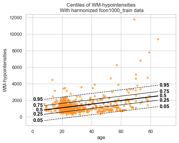
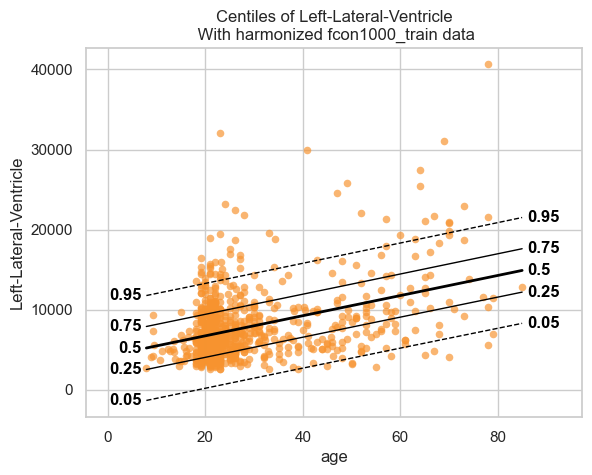
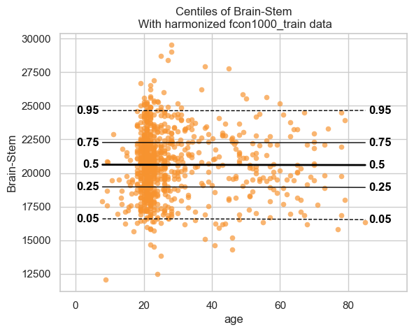
We see that the model fits the data reasonably well. We can do better, but that is a topic for another tutorial.

Showing the evaluation metrics

We also computed evaluation metrics for the model. Those are saved in the save_dir/results/statistics.csv file, but are also added to the NormData object as a new data variable.

# We can use the `get_statistics_df` method to get a nicely formatted dataframe with the evaluation metrics.
display(train.get_statistics_df())
display(test.get_statistics_df())

statistic	EXPV	MACE	MAPE	MSLL	NLL	R2	RMSE	Rho	Rho_p	SMSE	ShapiroW
response_vars
Brain-Stem	0.000004	0.006311	0.096330	-7.800671	1.418910	0.000004	2442.168242	-0.050426	1.390658e-01	0.999996	0.996466
Left-Lateral-Ventricle	0.162276	0.053828	0.401734	-8.440148	1.330158	0.162276	3877.069187	0.269669	7.905570e-16	0.837724	0.877568
WM-hypointensities	0.132905	0.068724	0.410158	-6.778665	1.345555	0.132905	760.501165	0.019769	5.621687e-01	0.867095	0.722254

statistic	EXPV	MACE	MAPE	MSLL	NLL	R2	RMSE	Rho	Rho_p	SMSE	ShapiroW
response_vars
Brain-Stem	-0.000274	0.014259	0.103240	-7.790895	1.525974	-0.000309	2692.120004	-0.105739	0.121292	1.000309	0.989058
Left-Lateral-Ventricle	0.175440	0.046296	0.430686	-8.443777	1.404512	0.171542	4168.272079	0.220610	0.001099	0.828458	0.898344
WM-hypointensities	0.150136	0.060741	0.444148	-6.693763	1.130787	0.143994	559.964146	-0.027495	0.687809	0.856006	0.972405

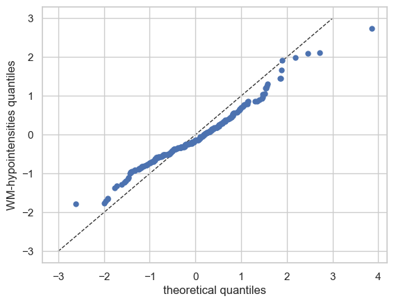
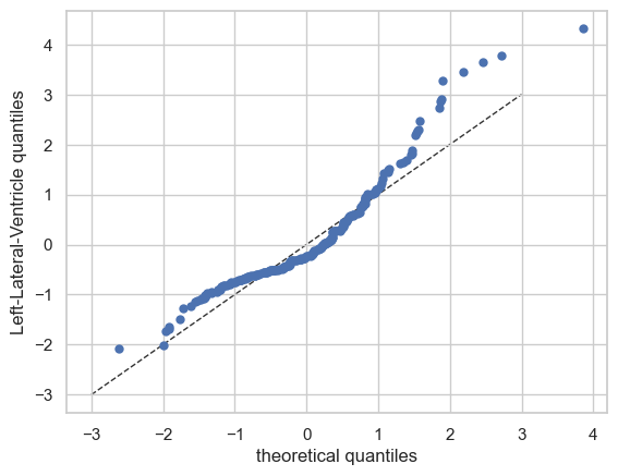
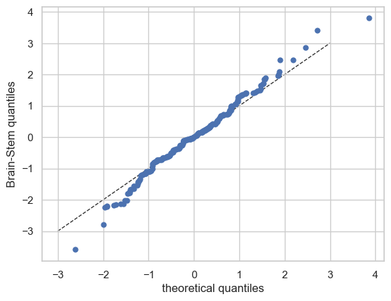
QQ plots

We also have a nice function to make QQ plots.

plot_qq(test, plot_id_line=True)

And those are the basics of Normative Modelling with the PCNtoolkit. We will go over some more advanced models in the next tutorials, but this should give you a good first impression.