Getting started with normative modelling
Welcome to this tutorial notebook that will show you the very basics of normative modeling. It’s like the “Hello World” of normative modeling.
Let’s jump right in.
Imports
import warnings
import pandas as pd
import matplotlib.pyplot as plt
from pcntoolkit import (
    BLR,
    NormativeModel,
    NormData,
    load_fcon1000,
    plot_centiles,
    plot_qq,
)
import pcntoolkit.util.output
import seaborn as sns

sns.set_style("darkgrid")
warnings.simplefilter(action="ignore", category=FutureWarning)
pd.options.mode.chained_assignment = None  # default='warn'
pcntoolkit.util.output.Output.set_show_messages(False)
Load data
First we download a small example dataset from github.
# Download an example dataset
norm_data: NormData = load_fcon1000()
# Select only these three features to model for this example
norm_data = norm_data.sel({"response_vars": ["WM-hypointensities", "Left-Lateral-Ventricle", "Brain-Stem"]})
# Train-test split
train, test = norm_data.train_test_split()
# Inspect the data
df = train.to_dataframe()
fig, ax = plt.subplots(1, 2, figsize=(15, 5))

sns.countplot(data=df, y=("batch_effects", "site"), hue=("batch_effects", "sex"), ax=ax[0], orient="h")
ax[0].legend(title="Sex")
ax[0].set_title("Count of sites")
ax[0].set_xlabel("Site")
ax[0].set_ylabel("Count")

scatter_feature = "Left-Lateral-Ventricle"

sns.scatterplot(
    data=df,
    x=("X", "age"),
    y=("Y", scatter_feature),
    hue=("batch_effects", "site"),
    style=("batch_effects", "sex"),
    ax=ax[1],
)
ax[1].legend([], [])
ax[1].set_title(f"Scatter plot of age vs {scatter_feature}")
ax[1].set_xlabel("Age")
ax[1].set_ylabel(scatter_feature)

plt.show()

Creating a Normative model
save_dir = "/Users/stijndeboer/Projects/PCN/PCNtoolkit/examples/saves"
model = NormativeModel(BLR(), inscaler="standardize", outscaler="standardize")
model.has_batch_effect
False
Fit the model
With all that configured, we can fit the model.
The fit_predict function will fit the model, evaluate it, save the
results and plots, and return the test data with all the predictions
added.
After that, it will compute Z-scores and centiles for the test set.
All results can be found in the save directory.
model.fit_predict(train, test)
<xarray.NormData> Size: 87kB
Dimensions:            (observations: 216, response_vars: 3, covariates: 1,
                        batch_effect_dims: 2, centile: 5, statistic: 11)
Coordinates:
  * observations       (observations) int64 2kB 756 769 692 616 ... 751 470 1043
  * response_vars      (response_vars) <U22 264B 'WM-hypointensities' ... 'Br...
  * covariates         (covariates) <U3 12B 'age'
  * batch_effect_dims  (batch_effect_dims) <U4 32B 'sex' 'site'
  * centile            (centile) float64 40B 0.05 0.25 0.5 0.75 0.95
  * statistic          (statistic) <U8 352B 'EXPV' 'MACE' ... 'SMSE' 'ShapiroW'
Data variables:
    subject_ids        (observations) object 2kB 'Munchen_sub96752' ... 'Quee...
    Y                  (observations, response_vars) float64 5kB 2.721e+03 .....
    X                  (observations, covariates) float64 2kB 63.0 ... 23.0
    batch_effects      (observations, batch_effect_dims) <U17 29kB 'F' ... 'Q...
    Z                  (observations, response_vars) float64 5kB 0.8681 ... -...
    centiles           (centile, observations, response_vars) float64 26kB 75...
    logp               (observations, response_vars) float64 5kB -1.254 ... -...
    Yhat               (observations, response_vars) float64 5kB 2.041e+03 .....
    statistics         (response_vars, statistic) float64 264B 0.1501 ... 0.9891
    Y_harmonized       (observations, response_vars) float64 5kB 2.721e+03 .....
Attributes:
    real_ids:                       True
    is_scaled:                      False
    name:                           fcon1000_test
    unique_batch_effects:           {np.str_('sex'): [np.str_('F'), np.str_('...
    batch_effect_counts:            defaultdict(<function NormData.register_b...
    covariate_ranges:               {np.str_('age'): {'mean': np.float64(28.2...
batch_effect_covariate_ranges: {np.str_('sex'): {np.str_('F'): {np.str_(...Plotting the centiles
With the fitted model, and some data, we can plot some centiles. There are a lot of different configurations possible, but here is a simple example.
plot_centiles(model, scatter_data=train)
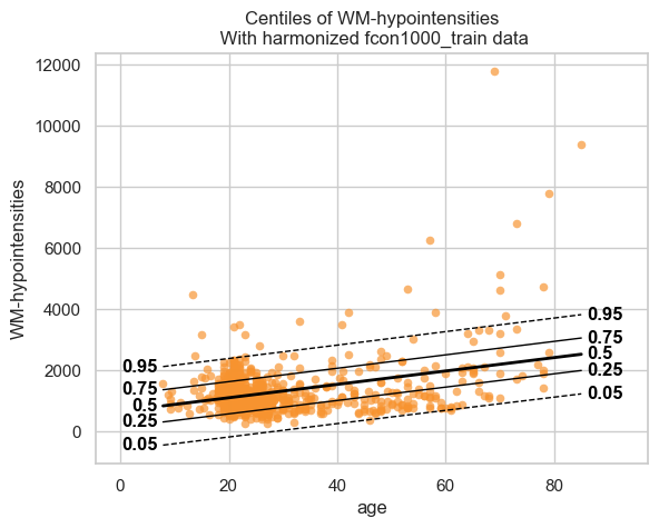


We see that the model fits the data reasonably well. We can do better, but that is a topic for another tutorial.
Showing the evaluation metrics
We also computed evaluation metrics for the model. Those are saved in
the save_dir/results/statistics.csv file, but are also added to the
NormData object as a new data variable.
# We can use the `get_statistics_df` method to get a nicely formatted dataframe with the evaluation metrics.
display(train.get_statistics_df())
display(test.get_statistics_df())
| statistic | EXPV | MACE | MAPE | MSLL | NLL | R2 | RMSE | Rho | Rho_p | SMSE | ShapiroW |
|---|---|---|---|---|---|---|---|---|---|---|---|
| response_vars | |||||||||||
| Brain-Stem | 0.000004 | 0.006311 | 0.096330 | -7.800671 | 1.418910 | 0.000004 | 2442.168242 | -0.050426 | 1.390658e-01 | 0.999996 | 0.996466 |
| Left-Lateral-Ventricle | 0.162276 | 0.053828 | 0.401734 | -8.440148 | 1.330158 | 0.162276 | 3877.069187 | 0.269669 | 7.905570e-16 | 0.837724 | 0.877568 |
| WM-hypointensities | 0.132905 | 0.068724 | 0.410158 | -6.778665 | 1.345555 | 0.132905 | 760.501165 | 0.019769 | 5.621687e-01 | 0.867095 | 0.722254 |
| statistic | EXPV | MACE | MAPE | MSLL | NLL | R2 | RMSE | Rho | Rho_p | SMSE | ShapiroW |
|---|---|---|---|---|---|---|---|---|---|---|---|
| response_vars | |||||||||||
| Brain-Stem | -0.000274 | 0.014259 | 0.103240 | -7.790895 | 1.525974 | -0.000309 | 2692.120004 | -0.105739 | 0.121292 | 1.000309 | 0.989058 |
| Left-Lateral-Ventricle | 0.175440 | 0.046296 | 0.430686 | -8.443777 | 1.404512 | 0.171542 | 4168.272079 | 0.220610 | 0.001099 | 0.828458 | 0.898344 |
| WM-hypointensities | 0.150136 | 0.060741 | 0.444148 | -6.693763 | 1.130787 | 0.143994 | 559.964146 | -0.027495 | 0.687809 | 0.856006 | 0.972405 |
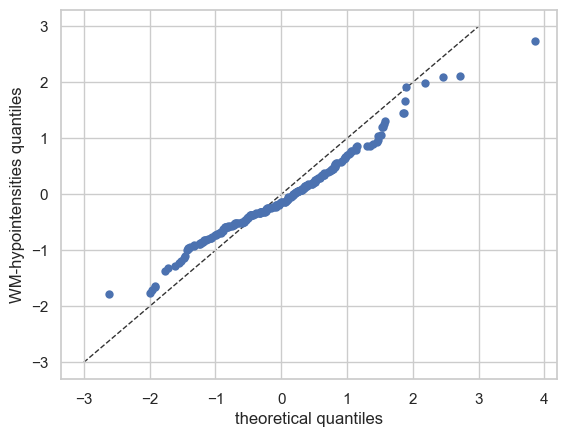
QQ plots
We also have a nice function to make QQ plots.
plot_qq(test, plot_id_line=True)


And those are the basics of Normative Modelling with the PCNtoolkit. We will go over some more advanced models in the next tutorials, but this should give you a good first impression.